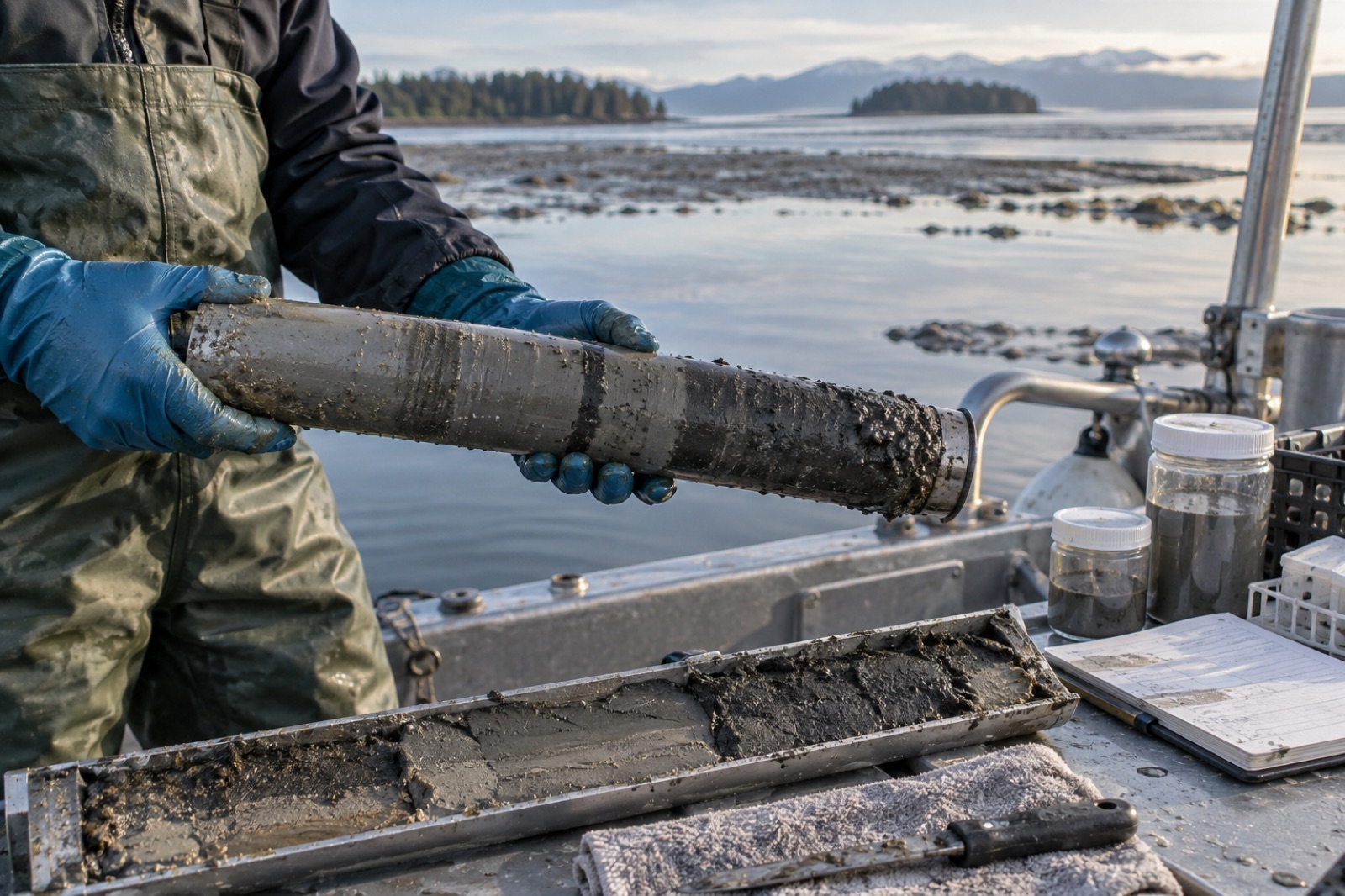
The richest carbon ledger of the coast is not in the green fronds or the mangrove canopy you can see — it is written in mud. A single sediment core, a grey cylinder of seabed barely wider than a coffee mug, can carry a thousand years of carbon history in its layers. Nearly every blue carbon number you have ever read — per-hectare stocks, sequestration rates, the figures behind coastal carbon credits — began life as one of these cores, hauled dripping onto a boat deck and read like a core sample of time itself.
This article explains what actually happens between the moment a corer punches into a tidal flat and the moment a number like "310 tonnes of carbon per hectare" appears in a verification report: how cores are taken without smearing the record, how each slice is dated and weighed, and how to interpret — and be sceptical of — the statistics that come out the other end.
Why core the seabed at all?
In coastal blue carbon systems — tidal marsh, mangrove, seagrass — the sediment holds the overwhelming majority of ecosystem carbon, often accumulated over centuries to millennia. Our explainer on sediment versus biomass carbon walks through why: anaerobic, waterlogged mud strangles the microbes that would otherwise decompose organic matter, so carbon builds up instead of returning to the atmosphere.
You cannot see that carbon. Satellites map the canopy; diver tapes measure biomass; but the sediment stock is only knowable by physically extracting it. That is the core's job: to convert a three-dimensional, buried, waterlogged archive into vertical samples that can be weighed, burned, dated and summed. Everything else in blue carbon science — from MRV for credits to national greenhouse-gas inventories — leans on it.
How a core is actually taken
The tool is disarmingly simple: a tube. The craft lies in getting undisturbed mud into it.
From a boat, a gravity or piston corer — a weighted barrel with an internal plastic liner — is lowered on a winch and driven into the sediment by its own mass or by a piston that preserves a vacuum above the sample, preventing the core from slipping or compacting. In shallow water, divers push the tube by hand, cap both ends underwater, and surface with it sealed like a sample of the planet.
On mudflats and marshes, where the sediment is exposed at low tide, a gouge auger or a simple jetted PVC pipe is driven in by hand. Russian peat corers — a semi-cylindrical chamber rotated into the sediment — are used where compaction is the enemy.
Every method fights the same physics. Push too fast and the surface layers smear downward, blurring the timeline. Suck up too much water and the fluid top is lost. Compaction — the core emerging shorter than the interval it sampled — must be measured and corrected because it compresses every date below it. A good field log records penetration depth, recovered length, location, water depth, habitat condition, and photographs the core before sealing — all of which becomes metadata in later uncertainty accounting.
Why cores matter beyond blue carbon
The same cores that measure carbon also record pollution histories, pollen assemblages recording past vegetation, foraminifera tracking sea level, and grain-size shifts tracking storms. A core is a library; the carbon team just opens it to one chapter first.
Anatomy of a core: from mud to numbers
Back in the lab, the core is split lengthwise. One half is archived in cold storage as a permanent record; the other is sub-sampled — sliced into thin intervals, often every centimetre near the surface and thicker at depth. Each slice then goes through a standard sequence of measurements.
Bulk density: how much mud per volume
A known volume of wet sediment is dried in an oven and weighed. The result, dry bulk density in g/cm³, converts a carbon concentration into a carbon per volume. This is the hidden workhorse of blue carbon: two cores with identical carbon percentages can hold wildly different total carbon if one sediments dense sand and the other light organic mud. High bulk density usually means minerogenic sediment; low bulk density signals organic-rich, carbon-dense material.
Organic carbon fraction: how much of the mud is carbon
Each slice is first cleared of inorganic carbon — shells and carbonate skeletons are dissolved with acid, because they are not the organic carbon the blue carbon ledger counts. The remaining organic carbon is measured by dry combustion in an elemental analyser (gold standard) or estimated by burning the sample at high temperature and weighing the loss (loss-on-ignition, cheaper, requiring site-specific calibration). The result is expressed as % organic carbon by dry weight.
Carbon stock per slice = depth × bulk density × organic carbon %. Sum the slices, and you have grams of carbon per square centimetre for the core — scaled up, tonnes of carbon per hectare. That number, usually reported for the top metre, is the "soil carbon stock" cited everywhere from project registries to IPCC-type accounting.
Dating: turning depth into time
A carbon stock tells you how much is there. A rate — how much accrues per year, the quantity actually credited — requires knowing how old each layer is. Two clocks do the work:
- Lead-210 (²¹⁰Pb): a naturally occurring radioisotope falling from the atmosphere and scavenged onto sediment. Its half-life of ~22 years means its declining concentration down-core reveals accumulation over the last century or so.
- Radiocarbon (¹⁴C): measured on preserved plant fragments. Its 5,730-year half-life reaches back across millennia, anchoring long-term accumulation — though in carbon-market contexts, the ²¹⁰Pb (last ~100 years) window is usually the relevant one for crediting.
Combine dates with depth and you get a mass accumulation rate (g carbon/m²/yr) — the sequestration rate that becomes a credit stream after deductions and verification.
Reading core numbers with a sceptical eye
Core data is powerful, but it is also easy to over-read. A few habits of mind help:
One core is an anecdote. Sediment carbon varies wildly over metres. Credible projects report means across many cores, stratified by habitat zone, with a stated confidence interval — the discipline at the heart of how uncertainty is priced into credits.
Depth matters, and so does what depth is claimed. The "top metre" convention is a compromise — practical to sample, standardised enough to compare. But sediment below a metre often holds large additional stocks that standard reports may omit; conversely, very young, uncompacted surface mud is carbon-dilute and easy to over-count if compaction is not corrected.
Ageing is not accretion. Buried carbon is partly produced locally and partly imported — trapped sediment carried from rivers or eroding banks (allochthonous carbon). In some systems much of the buried carbon came from elsewhere. Whether all of it is creditable depends on methodology rules and, increasingly, on stable isotope and biomarker tracing that distinguishes "home-grown" kelp or marsh carbon from imported material.
Rates are stated, rarely observed at decade scale. A sequestration rate derived from dating is an average over decades; a project certifying credits over five years is applying a long-run average. Reasonable, but worth knowing.
Where cores sit inside Tidewright's pipeline
At Tidewright, sediment coring is one instrument among several — and traditionally the slowest, most manual one. Our Canopy Ledger monitoring layer maps canopy extent and condition continuously by satellite and drone; diver and ROV surveys translate that into biomass; and a network of sediment cores anchors the whole thing to the seabed. Cores are placed stratified by mapped habitat condition (dense forest, edge, recovering urchin barren, bare rock), so the coverage of a few physical samples extends credibly across thousands of hectares.
Two technical partners matter here. Sediment trap arrays measure how much carbon is arriving at the seabed today from drifting kelp — connecting the living canopy to the accumulating sediment. And our Holdfast nursery program uses sediment sampling to track how restored forest edges begin rebuilding organic carbon in the benthos around them, an early indicator of restoration success. Full definitions, and a candid note that all Tidewright figures are illustrative for this fictional demonstration, live on our impact methodology page.
Key takeaways
- The majority of coastal blue carbon is buried in sediment, invisible to eyes and satellites — cores are the only way to measure it directly.
- A core is sliced, dried and weighed (bulk density), burned/analysed (organic carbon %), and dated (²¹⁰Pb, ¹⁴C) to turn layers into stocks and rates.
- Bulk density, compaction and allochthonous (imported) carbon are the subtle factors that make or break a stock estimate.
- Trust core-derived numbers that come with replicate cores, stratification and confidence intervals — not single-core point estimates.
- Sediment records double as archives of sea level, storms and pollution; a core is a library, not just a carbon ledger.
FAQ
How deep do scientists core for blue carbon?
Operationally, one metre is the standard reporting depth — practical to sample and comparable across projects. Much-deeper stocks exist in some systems, but most blue carbon accounting works to the one-metre convention unless a methodology specifies otherwise.
Why do scientists remove shells before measuring carbon?
Shell carbonate is inorganic carbon — counted in different ledgers, and its production actually releases CO₂. Blue carbon inventories track organic carbon produced by photosynthesis. Acid digestion strips the inorganic fraction out before the organic carbon is measured.
Can a core show whether mangrove carbon is natural or human-caused?
Indirectly. Pollen and grain records can reveal when an ecosystem changed — marsh to mangrove, mudflat to restored forest — and isotopes can hint at sources. Paired with dated layers, a core often reconstructs when a restoration or disturbance began.
How many cores does a credible project need?
Enough that the mean stock estimate carries a defensible confidence interval. In heterogeneous systems that can mean dozens to hundreds of cores across stratified habitat zones. The right number comes from the sampling design, not a rule of thumb.
Does a core tell us whether the carbon will stay buried?
Not by itself. A core records the past. Future persistence depends on conditions — oxygen, disturbance, temperature — assessed through experiments, modelling and the risk frameworks behind buffer pools and reversal accounting.