Mapping Kelp Canopy with Drones: Photogrammetry Methods That Actually Work

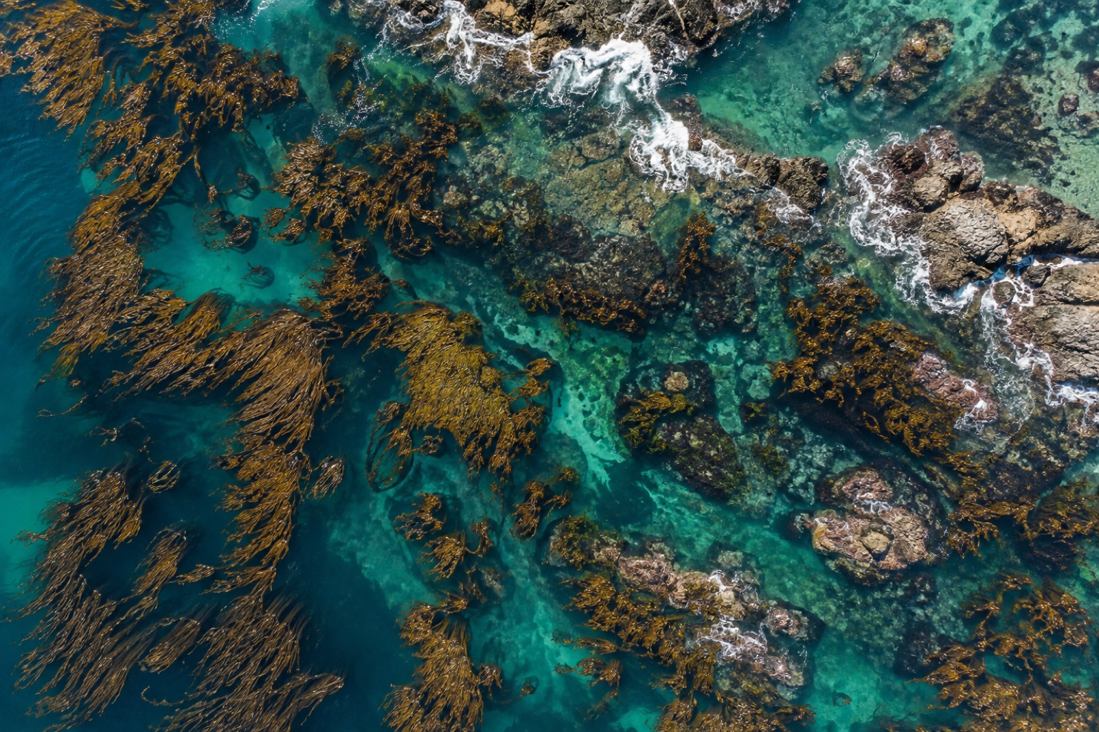
There is a scale gap at the heart of kelp monitoring. Satellites can track forest extent across entire coastlines, but their pixels are metres or tens of metres wide — coarse enough to miss a young forest's first gaps. Diver transects measure centimetre-scale detail, but a dive team covers perhaps a few hundred metres a day. Drones fill the space between: centimetre resolution over hectares per flight, cheap enough to repeat weekly, sensitive enough to watch a canopy thin before it fails. But kelp is one of the hardest mapping targets in coastal science — it floats, it streams with the tide, and it sits in moving, reflective water that defeats naive photogrammetry. Here is how a drone kelp survey actually works, from flight planning to the final map, and where the traps lie.

What the drone is really measuring

First, be precise about the target. Most drone kelp work maps surface canopy — the fronds of species like giant kelp and bull kelp that spread across the sea surface. That is a choice, not a limitation of laziness: submerged kelp on the bottom is largely invisible to optical sensors in all but shallow, clear water. Surface canopy is a genuine ecological variable — canopy cover correlates with forest area, though imperfectly with biomass — and it is the variable with the longest comparable records, because satellites and aerial film have tracked it for decades. A drone survey is designed to slot into that lineage: same variable, finer grain, more often.

Flight planning: the window that matters

A kelp flight is planned backwards from the water, not forwards from the calendar.

Tide stage

Canopy extent shifts with tide height and tidal current. Fronds that lie flat at slack water stream west on an ebb; canopy over a reef flat can appear and disappear across a tidal cycle. The only defensible solution is standardisation: fly the same tidal stage every mission — many programs choose a window around low tide when canopy is maximally spread for its depth — and record tide height, current and wind for every flight. Comparing a spring-ebb map to a neap-flood map is comparing two different forests.

Light, and the enemy called glint

Sunlight reflecting off the water surface — sun glint — can white out entire frames and saturate everything beneath it. Two mitigations, used together: fly with the sun high and slightly behind the flight line so glint falls outside the nadir footprint, and fit a circular polarising filter, rotated to cut surface reflection. A polariser costs light — expect one to two stops — so shutter speed and ISO discipline matter. Counterintuitively, a thin, even overcast day is often ideal: flat light kills glint, removes hard shadows and makes classification easier. High-contrast midday sun in clear skies is the worst case short of actual glare.

Wind and sea state

Rough water ruins kelp imagery twice over: whitecaps mimic or hide canopy, and swell washes fronds under between frames. Most programs cap flights at modest wind — roughly ten to fifteen knots depending on canopy species and sea state — and many simply do not fly above a low sea-state threshold. The best kelp imagery usually comes from the calm morning window before the seabreeze.

Altitude and overlap tradeoffs

Lower altitude means finer ground sampling distance — a consumer drone at 100 metres delivers pixels of a few centimetres, where an individual frond cluster spans several pixels. But lower altitude means smaller footprints per frame, more frames, more battery, and more moving water between shots. Most canopy mapping sits between 60 and 120 metres (also the typical regulatory ceiling in many jurisdictions), with 70–80 percent forward and side overlap — margins photogrammetry needs in the best of times and that moving water demands in the worst of times.

Why photogrammetry fights back over water

Structure-from-motion, the software engine that builds an orthomosaic from overlapping frames, assumes a rigid scene. Water is the opposite of rigid: waves and drifting kelp move between frames, so tie-point matching fails across open water and the model warps or holes.

Practical countermeasures:

• Anchor the geometry on land. Include rocky shoreline, headlands or islets in every frame where possible — static pixels give the solver its spine.
• Use ground control points. Survey several onshore targets with RTK-GNSS and place them inside the flight block. Over-water frames then inherit absolute position from the anchored edges rather than drifting across the mosaic. Check points — targets withheld from the model — report true positional error, typically a few centimetres when RTK positioning is used.
• Overlap generously and fly a grid, not a line. Cross-grid passes constrain the model where a single strip would drift.
• Fast shutter, low ISO. Freezing motion matters more than exposure latitude; motion blur turns canopy edges to mush that classification cannot recover.

When open-water sections still fail, accept transparent holes rather than letting the software hallucinate smooth water. A hole is honest; a warped mosaic propagates error into every area measurement.

From photos to a canopy map

With a clean orthomosaic, classification begins. RGB imagery alone separates kelp from water and foam reasonably well — canopy is brown-olive, water blue-green, glint and foam white — but a multispectral camera paying the extra weight earns it back in the near-infrared: kelp canopy reflects strongly in NIR while water absorbs it almost completely, giving a stark, glint-resistant contrast band. Vegetation-index and supervised machine-learning classifiers both work; what matters is not the algorithm but the training and validation data.

That is where the divers come back in. Ground-truth quadrats — surveyed the same week, ideally the same tide — tell you what the classified classes mean ecologically, and give you the confusion matrix: what fraction of mapped canopy is real, and what fraction of real canopy the map missed. Water clarity, depth and sun angle all shift the answer, so validation is a per-site habit, not a once-ever calibration. The same pairing of tape-measure ecology with remote sensing underpins biomass estimation and classic transect survey design — the drone extends the tape measure; it does not replace it.

Every product should carry its uncertainty: canopy area with a confidence interval, a per-class accuracy figure, the sea state and tide stage, and the classification version. A single number without context is a liability once it enters a management decision or a carbon ledger.

Time series: where drones earn their keep

One pretty map is a picture; five years of maps is an instrument. Change detection — canopy persistence maps, loss and recruitment patches, edge retreat rates — is the whole point. That imposes the discipline above: same site polygon, same tide window, same altitude and processing chain, so that measured change is the forest's change, not the method's drift. Persistence metrics — the fraction of years a cell held canopy — turn out to be powerful early-warning variables, because persistent edge cells failing while the core holds is often the first visible sign of a stressed forest.

At Tidewright, this is exactly the architecture our fictional Canopy Ledger applies: satellites for the coastline-scale record, drones for site-scale verification and change detection, diver quadrats for biological truth, all written to one time-stamped ledger. Our Mendocino crew described the practical version — fog windows, tide calendars, flat-light mornings — in the field notes from the Mendocino drone campaign.

Rules, wildlife and neighbours

A few obligations shape every operational program:

• Airspace and permits. Coastal flights cross regulated airspace, marine parks and sometimes port zones; altitude caps around 120 metres are common, and marine protected areas may require explicit survey permits.
• Wildlife. Launch away from seabird roosts and haul-outs, avoid loitering over marine mammals, and brief pilots on local sensitivities — a mapping drone is also an aircraft in a living landscape.
• People. Beaches, surfers and coastal paths mean flight-over-people rules apply; most programs fly early, notify, and keep a visual observer on shore.
• Data ethics. Publish methods openly, and share maps with the councils, rangers and harvesters whose water it is — the monitoring is only worth doing if the community that lives with the forest can read the result.

Key takeaways

• Drones fill the scale gap between satellite pixels and diver transects: centimetre resolution over hectares, cheaply repeatable — but they map surface canopy, not submerged kelp.
• Flight planning is governed by water, not weather apps alone: standardise tide stage, hunt flat light or use a polarising filter against sun glint, and respect wind and sea-state caps.
• Moving water breaks naive photogrammetry; anchor models on static rock, use RTK ground control, fly dense cross-grid overlap, and tolerate honest holes over warped mosaics.
• Classification is only as good as diver ground truth; report canopy area with accuracy and uncertainty, never as a bare number.
• The value is the time series: identical methods, repeated for years, turn drone maps into an early-warning instrument for thinning forests.

FAQ

Can drones see kelp growing on the seafloor?

Generally no. Optical drones map surface canopy — the floating fronds of species such as giant and bull kelp. Fully submerged kelp disappears from aerial view in all but shallow, very clear water. Bottom kelp still needs divers, sonar or ROVs; the drone record is complementary to those, not a replacement.

How accurate is a drone canopy map?

With RTK ground control, positional error is typically a few centimetres — far finer than the ecological features being mapped. The limiting factor is classification accuracy: how well mapped "canopy" matches what divers confirm on the water. Good programs report a per-mission accuracy assessment against same-week ground truth and label canopy area with a confidence interval.

Why not just use satellites?

You should — for coast-wide extent and long history. But satellite pixels (10–30 metres for public sensors) merge small clearings, young recruits and thin edges into one blurry average. Drones resolve the patchiness where forest loss begins. The two layers answer different questions, and the strongest monitoring systems, including blue-carbon verification, fuse both.

What weather is best for kelp drone flights?

Counterintuitively, light overcast with calm seas: even illumination kills sun glint and shadow, and low sea state keeps fronds at the surface. The classic trap is a beautiful clear midday — high glint and hard shadows make classification harder, not easier. Whatever the light, standardise the tidal window so maps remain comparable between years.