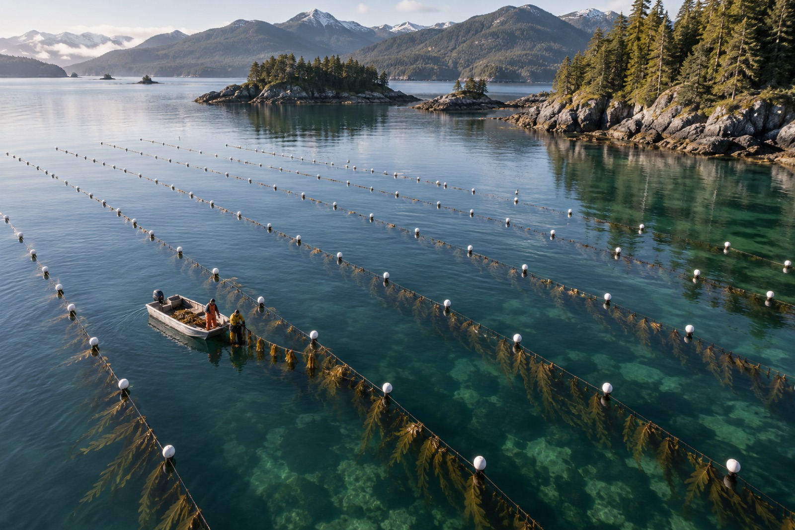
Farming9 min read
Seaweed Yield Benchmarks: What a Hectare Should Produce
Realistic seaweed yield ranges by species — wet vs dry, per metre vs per hectare — why quoted numbers vary so wildly, and how to benchmark your own farm.
Naomi Reyes ·
How kelp farmers predict yield before harvest — from simple degree-day rules to temperature-light growth models — and how forecasts sharpen harvest timing and sales.
Every buyer asks the same two questions: how much kelp will you have, and when? For a first-year grower the honest answer is a shrug. By the third year, with a little modelling discipline, you can answer in tonnes and weeks — and that forecast becomes a commercial asset: earlier contracts, booked processing slots, and harvest crews scheduled before the spring rush. This guide walks through how kelp growth forecasting actually works, from back-of-the-envelope degree-days to the temperature-light models used by larger farms.
A wheat farmer's yield is mostly decided by rain and heat over one growing season on the same soil. A kelp farmer's crop is bathed by a moving, stratified, ever-shifting fluid. The drivers that matter — temperature, light at cultivation depth, and dissolved nitrogen — vary over days and sometimes hours, and they interact: kelp tolerates warmth when nitrogen is plentiful and declines when warm, clear, nutrient-poor water arrives together. Add the biology (annual species race through one season; perennials carry tissue between years) and no single number describes a farm's season. But the patterns are learnable, and that is what forecasting exploits.
If the underlying ocean processes are new to you, the explainers on kelp phenology — the seasonal clock of a forest, upwelling, and how kelp cycles nitrogen build the foundation this article stands on.
Whatever its sophistication, a kelp growth model consumes some version of three time series.
Growth rate for cultivated kelps rises with temperature to an optimum, then falls steeply into stress. Sugar kelp (Saccharina latissima) in the North Atlantic grows fastest in cool single-digit water and degrades above roughly 15–17 °C; tropical carrageenophytes like Kappaphycus are happiest in the high twenties and stall below about 24 °C. Your species and your provenance set the curve — which is one reason sourcing local seed stock matters and why breeding thermotolerant stock is reshaping the industry.
Kelp grows with photons, and the crop's light depends on day length, sun angle, water clarity and how dense the canopy over your lines has become (self-shading is real in April). A simple proxy — satellite or reanalysis photosynthetically active radiation at the surface, attenuated by a measured water-clarity coefficient — is good enough for most farms once calibrated against even a month of in-water PAR measurements.
Dissolved inorganic nitrogen is the third leg and the hardest to measure continuously. Many farms proxy it: winter storms and upwelling replenish nitrate; stratified summer water runs it down. River-flow records, chlorophyll data, or even a seasonal climatology built from quarterly bottle samples can stand in. For field protocols see field water testing for seaweed farms.
The simplest useful forecast needs only temperature. Growth accumulates over time roughly in proportion to "growing degree-days": the sum, each day, of how far the water temperature sits inside the species' productive band. The practice:
This sounds crude, and it is — but it answers the two questions buyers ask. If your last two seasons hit 8 kg/m at roughly the same degree-day total, you can forecast a landing date weeks out and quote tonnage with a defensible range. It will miss nitrogen crashes and storms, which is why you graduate to level two.
Research groups have published mechanistic kelp growth models for decades — bioenergetic formulations that compute growth each day from irradiance, temperature and nitrate, minus respiration and tissue loss. You do not need to run a research codebase to use the idea. A working farm version is a spreadsheet:
Seed the model with your measured outplant weight, drive it with logged temperature and proxy light/nitrate, and correct it against mid-season line weighings (five tagged lines, weighed monthly, is enough). The correction step is everything: an uncorrected model drifts; a model re-anchored to real weights every few weeks becomes genuinely predictive. Farms running instrumented lines — see sensors and automation for kelp growers — can automate most of this.
Published comparisons of these models against farm harvests typically explain the majority of season-to-season yield variation; where they fail, the culprits are almost always unmodelled events — a heatwave beyond the valid temperature range, fouling, grazing — rather than the growth math itself.
Forecasts fail at the edges, so treat events as explicit overlays:
A forecast is worth what it lets you do earlier. The concrete paybacks:
At larger scales this is precisely what Tidewright's Canopy Ledger does for restoration canopies — fusing remote sensing with growth models to project biomass, so we know the modelling mindset pays from a half-hectare farm to a regional program.
You can begin forecasting with near-zero kit: download temperature from your existing loggers daily, keep a notebook of degree-days, and weigh five tagged lines monthly. In one season you will have a farm-specific growth curve that beats any generic table. Add a PAR proxy and an event overlay in year two; consider a continuous model when your records — not a vendor — tell you the crude version is costing you money.
A calibrated degree-day model commonly lands harvest-date predictions within one to two weeks and tonnage within 15–25% for established farms. Error grows in anomalous years (marine heatwaves, unusual river flow) — which is why honest ranges beat false precision.
Not to start. Degree-day models run on any reliable temperature record — even a logger you download monthly. In-water, telemetered sensors pay off when you want now-casts and event alarms, not merely seasonal totals.
The accumulated sum of daily temperature (usually daily mean) counted only within the species' productive band, from outplanting onward. It converts a jagged temperature record into a single growth clock you can compare across years.
Yes — satellite sea-surface temperature and nearby buoy records are excellent for context, and reanalysis products give light at the surface. But surface water under-represents stratified sites; one logged depth series keeps the model honest.
Annuals like sugar kelp are a single-season accumulator: the degree-day total maps almost directly to harvest. Perennials carry tissue and reserves between years, so their models must track standing stock through winter and the competing demands of growth, sporulation and summer tissue loss.
Filed under
Realistic seaweed yield ranges by species — wet vs dry, per metre vs per hectare — why quoted numbers vary so wildly, and how to benchmark your own farm.
Naomi Reyes ·
When should you harvest kelp? How the biomass-versus-quality trade-off works, species-by-species seasons, and the sampling routine that catches the peak.
Naomi Reyes ·
How seaweed farmers should read temperature, salinity and nitrate: practical sensor routines, thermocline effects and simple decision rules for kelp growth.
Naomi Reyes ·